

Precise or Accurate? Your Test and Measurement Instruments Need to Be Both!
on
In writing technical articles, we often risk losing some language accuracy, and this becomes more evident in rigorous fields — such as metrology — where each term has a very specific usage and, generally, inappropriate terminology is not well-tolerated.
Measurements
A measurement is, by definition, a numerical relationship resulting from the comparison of a given quantity to another, homogeneous to it and of known value, considered as a reference.
Regardless of the unit of measurement, this measurement, comparison, and the resulting calculations cannot be error-free. Error is inherent to measurement; it can be reduced, but not eliminated. What can be done — to live with it — in the technical and scientific sphere, is to quantify its magnitude and consider it within the context of the overall measurement process.
Generally, in the T&M field, quality pays: The finest and most expensive measuring instruments can help reduce the margin of a measurement error, thus improving the quality of our work. However, this comes at a cost; technicians and engineers must evaluate, before purchase, the quality of the instrument they are going to buy, perhaps resorting to trade-offs between price and performance.
Terms such as precision, accuracy, repeatability, long-term stability, sensitivity, resolution, readiness, and full-scale value have become commonly used and can help one make a choice among the plethora of the devices available off the shelf. However, in this scenario, two of them are the most illustrious victims: precision and accuracy, which are often used interchangeably and improperly (which does not necessarily cause much harm).
An Initial Definition
What do Accuracy and Precision really represent in metrology? Let’s start with two concise definitions:
- Accuracy: An instrument is defined as accurate if it is capable of providing readings consistently as close as possible to a reference value, or true value.
- Precision: An instrument is defined as precise if it is capable of providing readings that correlate as consistently as possible with the average value of the readings taken.
Having briefly defined them, we must note something important: With only one reading available, we can define the accuracy of an instrument (albeit approximately), but not its precision, for which we need an average value or, possibly, a number such that the calculations are statistically significant and provide a reliable result.
Before going further into detail, however, it will be worth spending a few words defining the concept of error.
Measurement Errors
In a single measurement, error can be defined as the difference between measured value X and true value θ (or reference value, if we assume it as being true) of the quantity under consideration. In this case, it’s generally defined as an absolute error, or η = X - θ.
The absolute error value is merely part of the information, as it doesn’t give us any clue as to the ratio of this error versus the quantity we are comparing. That’s why the magnitude of an error is often expressed as the ratio of absolute error η to the true value θ, thus defined as relative error, or ε = η / θ.
This error can be calculated only if the reference value, θ, is known. The value of ε is usually expressed as a percentage, by multiplying it by 100. For this reason, the percentage error is generally indicated for each individual range of a measuring instrument.
Types of Error
There may be many causes of errors in an experimental measurement, including procedural ones (operator errors, for instance). With analog measuring instruments, in particular, operator error becomes more significant, as described in the "Analog vs. Digital Readout: Resolution Matters!" section of this article.
Here, however, we will assume that there is no operator error and that any errors present depend mainly on random factors and on the device’s features.
We may divide these errors into two macro-categories:
- Systematic errors, which constantly bias measurements in one direction. This type of error can be reduced or eliminated, in some cases. It mainly affects the accuracy of an instrument.
- Random errors, determined by the technical properties of the instrument, the quality of its design and on the components used, and by all the unpredictable and/or uncontrollable events that might occur during measurement. This type of error, which affects mainly the precision of an instrument, cannot be eliminated, but it can at least be estimated by repeating the measurement several times and analyzing the resulting statistics.
In an electronic measuring instrument, systematic errors can be caused, for example, by long-term variations in the characteristics of the components used (derating), or by short-term variations, such as an out-of-range device operating temperature. On higher quality equipment, one or more calibration options are usually provided to reduce the magnitude of these errors — either via hardware or in software.
Random errors, on the other hand, can be introduced by electromagnetic interference (EMI) conducted by probe cables, or by the inherent instability or poor quality of the signal conditioning and/or sampling front-end. They can be partially reduced by shielding, but nothing can be done to correct a design that is fundamentally deficient or poorly functioning.
Analog vs. Digital Readout: Resolution Matters!
The resolution of a measuring instrument is the smallest variation in the measured quantity that the device can reliably detect and display.
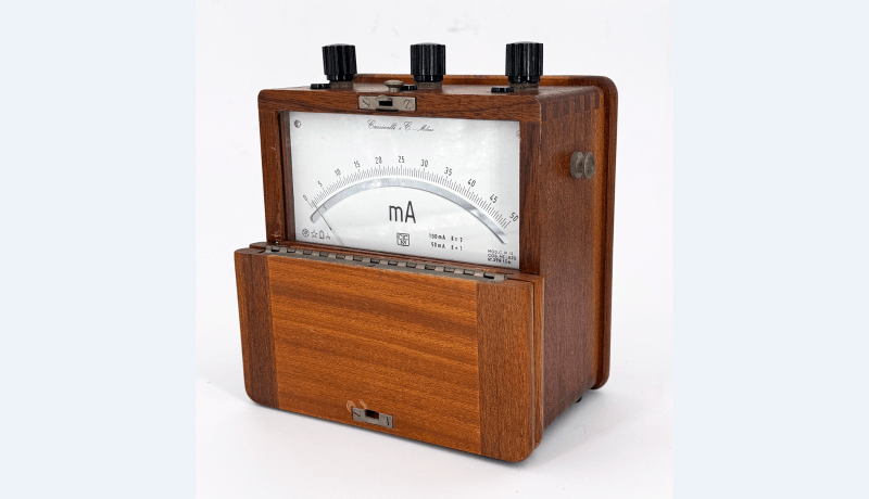
In the example in the image, a vintage Cassinelli & C. analog milliampere meter (circa 1960) and a latest-generation Siglent SDM3055 digital multimeter (2024) are connected in series to a current generator set at 30 mA. The upper image shows the 0…50 mA dial of the vintage instrument — whose accuracy, BTW, is absolutely remarkable, despite being more than 60 years old! — with 1 mA unit large divisions and 0.5 mA small divisions. Thus, the resolution of this instrument is 0.5 mA (500 µA).
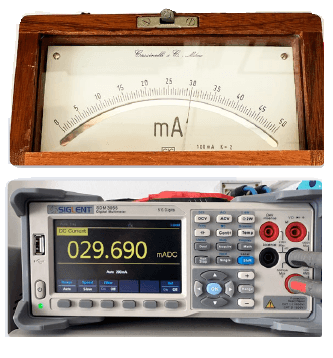
Here, the critical aspect is in assessing (optical targeting) the position of the needle in the areas between the divisions, with evaluations that are unavoidably personal, arbitrary and widely variable from operator to operator.
With the digital instrument, the display gives a reading of 29,690 mA on five digits — where the least significant digit represents the smallest quantity that the instrument is capable of measuring and displaying, i.e., 0.001 ma (1 µA). It goes without saying that resolution does not allow for any conclusions about accuracy or precision!
A First Practical Example
Let’s suppose to have 4 multimeters on our laboratory shelves and we want to check their performance in terms of reliability. In the lab, we have a high-end reference current generator available, and we set it up for a preliminary go-no-go test on one of those instruments.
To run the test, we set the current generator to 2.000 A, and we consider this value as true value, reference value, or θ.
Suppose that our first (and only) reading from that multimeter — from now on, defined as measured value, or X — indicates 2.0052 A. Then, as anticipated, we have an absolute error:
η = X − θ
η = 2.0052 - 2.0000 = 0.0052 A
Knowing η, we can then calculate relative error ε, which, expressed as a percentage, will be:
ε = (η / θ) × 100
ε = (0.0052 / 2.0000) × 100 = 0.26%
This figure represents a dimensionless number (i.e., without an associated unit) and means that our multimeter, in this specific reading and selected range, shows a relative error = 0.26%.
Building Statistics
The single measurement we’ve done so far on the first of our multimeters does not tell us much about the overall reliability of our instrument, nor does it allow us to determine whether it is affected by systematic errors, random errors, or both. So, for more meaningful insights, we take the matter more seriously and build up four databases of measurements.
We perform 100 consecutive readings on each multimeter, taking care not to vary the test conditions between one measurement and the next on any of the instruments. Each one of the measurements generates a Xn value.
Then we calculate the arithmetic mean of those readings and define it as the average measured value µ (with n = 100, in this case):
µ = (X1 + X2 + X3 … + Xn) / n
Knowing µ, however, is not sufficient; although it gives us some clues about the average accuracy, it does not allow us to quantify the error’s random component, thus preventing us from determining the precision.
Therefore, on the same acquired data, for each of the four databases, we assume that our measurements follow the law of normal distribution and calculate the standard deviation, σ, of readings X1…X100, using the following formula:
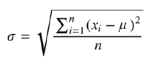
So, we can check how far the readings fall from the mean value obtained previously.
If you are not familiar with the concept of standard deviation, you can either take a look here or, for a more formal, mathematical approach, here. You may also take a look at "The Gaussian Distribution, in Short" section of this article.
The Gaussian Distribution, in Short
Often in science, the most important discoveries are the result of a combination of the study of several scientists. This is the case of the Gaussian Distribution, whose concept arose from various observations, starting in the late 1700s with Laplace’s fundamental central limit theorem, to follow with the insight of Abraham de Moivre who noticed that as the number of events increased, their distribution followed a rather smoothed profile, until the work of Carl Friedrich Gauss who defined the formula for calculating the curve that later took his name.
An interesting historical overview describing this course of study, which is the basis of modern statistics, can be found here.
Figure A illustrates a typical Gaussian distribution curve. In a normal distribution, within the analyzed sample there are values that symmetrically approach the µ value — the arithmetic mean of all the data — with a greater frequency than others, and this frequency contributes to giving the curve its characteristic bell-shaped form.

The area below the curve represents the distribution of the sample data. The Y axis indicates the frequency with which data of the same value occurs.
The distance between µ and the inflection point of the curve (where the curvature change in the other direction) represents what is commonly referred to as standard deviation or sigma (σ), root-mean-square deviation, or root-mean-square error.
In other words, sigma can be considered as an index of the dispersion of our data in respect to the average µ. Sigma and precision are inversely proportional, i.e. when the dispersion of the data decreases, their precision increases and the Gaussian curve becomes peakier. Conversely, with high sigma values, the curve becomes particularly flat and its base gets wider.
An empiric rule that’s commonly applied to a standard distribution curve states that the sample data have a 68.26% probability of falling in the [-σ…σ] interval (blue area, see Figure A), 95.44% in the [-2σ…2σ] interval (blue + purple areas) and 99.73% in the [-3σ…3σ] (blue + purple + green areas).
Sigma is not a dimensionless quantity, rather, it assumes the unit of measurement of the quantity under consideration (in the case of our four multimeters example it is ampere/A).
Interpreting Data
Multimeter 1
With the hundred measurements taken with multimeter 1, we calculate the respective average value µ and standard deviation σ as mentioned above. The resulting chart is shown in Figure 1. The curve shows the normal distribution of measurements around the mean value, µ, which for this instrument was found to be µ = 1.9. The plot of the distribution around µ is very “sharp,” indicating a high concentration of measurements with values very close to the average. However, this is distant from the true value θ = 2. The value δ = (µ − θ) = −0.1 is the expression of the average inaccuracy of this instrument.

It just needs to be calibrated using a reference instrument,
since its δ component is not negligible.
This is a typical case in which calibration of the instrument can help to reduce even substantially this error component, lowering δ to negligible values (close to 0) and restoring its expected accuracy.
The interval between the two worst readings (the base of the bell-shaped curve, indicated by the red arrow) is also referred to as the maximum measurement uncertainty. In measurements, uncertainty and precision are inversely correlated.
With σ = 0.042 A, (i.e. a standard error of ±2.2% on average µ), it can then be concluded that the instrument is precise, but being the systematic component of the error (δ = −0.1 A) high, it’s not accurate, with an average error = −5% to reference.
Multimeter 2
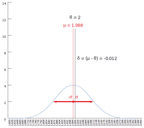
The chart of the second multimeter (Figure 2) shows a drastically different scenario. The mean value µ of the readings was found to be = 1.998, but the maximum measurement uncertainty of this instrument is far greater than multimeter 1.
useless by the significant error in precision.
With σ = ±0.116 A (±5.8% error on average µ), the random component of the error is large, with highly distributed (not concentrated) measurement values. Since it cannot be completely corrected, this random error component makes multimeter 2 unprecise, although its apparently astonishing accuracy δ = −0.012 A (−0.6% error on reference) might be misleading us.
All in all, a very accurate yet widely imprecise instrument that cannot be used in the laboratory, as the probability of obtaining unrealistic measurements is high. Using a different, yet common terminology, this instrument shows a very low repeatability, a synonym for precision.
This case shows how accuracy alone is not enough for obtaining a trustworthy measurement.
Multimeter 3
The situation with multimeter 3 is even worse, if that’s even possible. The graph of Figure 3 indicates a calculated mean value µ = 2.15, with δ = 0.15 A (+7.5% error on reference) that could well be significant on its own. Furthermore, with σ = ±0.19 A (±8.8% error on average µ), the distribution curve reveals a random error with an extremely flattened curve. The overall uncertainty is so great that it falls off the chart on the right-hand side. So, this third instrument results coarsely unprecise and unaccurate.

reference, worsened (if possible) by a widely spread uncertainty (very high σ).
Multimeter 4
The plot of the fourth instrument (Figure 4) appears to be the best of the series. The error distribution is concentrated on the mean of µ = 2.006, the resulting δ = 0.006 A (+0.3% error on reference value) can be considered as negligible and the value of the standard deviation σ = ±0.04 A (±2% on average µ) is low. The conclusion that can be drawn is that this is both a precise and accurate instrument, and because of its features, it can also be defined as exact.

and ±2% on precision, it will still be useful on the workbench.
A More Handy Representation
For a more practical depiction, the summary table in Figure 5 may be useful. In it, the above examples’ measurement distributions are represented on four targets. This is a widely used example in these cases, because of the very immediacy of its interpretation. In addition, the green and blue frames indicate the systematic and random error components’ areas, partially overlapping, in the worst case — multimeter 3, which is affected by high levels of both.
Ideally, the Cartesian axes could be superimposed on this drawing, where the Y axis represents precision, the X axis accuracy, and the straight line function Y = X in the first quadrant is the exactness of measurement, i.e. the combination of both.
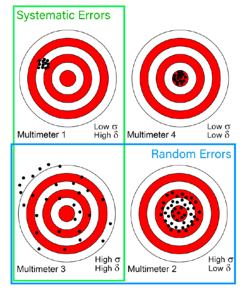
In the four targets, the diameter of the perforated areas represents
the dispersion (σ, the reciprocal of precision), while their distance from the
center (δ) indicates inaccuracy. Multimeter 4 is not error-free, but the two
error components, systematic and random, are far lower.
Reference Value or True Value?
At the beginning of this article, we wrote that we considered the reference value to be the true value. This is because we relied on the characteristics of our reference current generating instrument, considering it to be exact for our standards.
In reality — I’m sorry to disappoint you — the true value of any quantity exists, but it is unknown and inaccessible, given that every measurement is subject to an uncertainty level of greater than 0.
In other words:
- The true value is perfect, but only theoretical: impossible to determine exactly.
- The reference value is the best value available, and is used as a (local) standard in practical measurements.
The task of metrology is specifically to bridge, as far as possible, the distance between the true value and the measured value.
This distance is narrowed by using different standards, of increasingly higher level of accuracy, which constitute the so-called traceability chain of a measuring instrument. This, and many other detailed aspects of acquisition and reading errors inherent in electronic measuring instruments, will be the subject of a future article. Stay tuned!
Editor's Note: This article (250046-01) appears in the May/June 2025 edition of ElektorMag.
Questions or Comments?
Do you have technical questions or comments about this article? You can write to the author at roberto.armani@elektor.com or contact the editorial team at editor@elektor.com.


Discussion (1 comment)
Thack 6 days ago
Accuracy is how close the reading is to the true value. Accuracy is achieved by calibration.
Precision is how many digits (or equivalent) are used to display the measured value.
Repeatability is how consistent the displayed value is for a fixed true value.
For example, I might say: "I am 21 years, three months, one week, two days, 14 hours, 23 minutes and 10 seconds old.". That would be a highly precise but highly inaccurate description of my age.