Trying Out the NanoVNA V2 Vector Network Analyzer

What is the NanoVNA V2?

A Vector Network Analyzer (VNA) consists of a tunable high-frequency generator and a synchronously tuned receiver. The receiver measures the amplitude and phase of the signal at each point. This allows you to measure the real part of the signal and the imaginary part, or magnitude and phase angle, which together can be represented as a vector, hence the ‘V’ in VNA. ‘Network’ refers to any circuit with resistors, capacitors, and inductors. The VNA has two ports, an output and an input. You can place, for example, a bandpass filter between them to measure its frequency response.

I first saw such a device many years ago when I visited a friend who worked as an RF technician at a TV transmission tower. He had an older unit at home since his workplace had acquired a newer one. It was a huge, heavy box packed with tubes. At the time, I wasn’t convinced of its practical use. We wanted to build a resonant circuit for a specific frequency in the shortwave range to receive a DRM transmitter. Because the VNA’s ports had an impedance of 50 Ω, we had to add coupling windings to the resonant circuit. We managed to do it, but I thought it was too much effort. I preferred using a dip meter or estimating the coil turns and fine-tuning with the core screw.

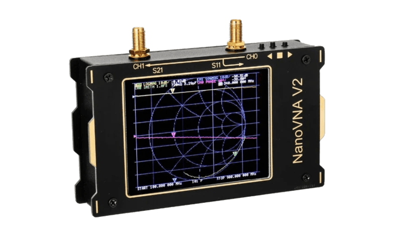
The Compact NanoVNA V2

Today, there are small, compact, and affordable devices like the NanoVNA V2 with excellent features. I have now come to appreciate the advantages of such a device. However, the journey wasn’t easy, as I initially found the display and many menu functions very confusing. I’m still not fully through with it, but I found software that allows me to control everything from my PC: VNA View.

 

First, you need to connect the USB cable and select the appropriate COM port in the Device menu. Once the connection is established, the display on the NanoVNA V2 goes blank, and it shows the message USB MODE.

Practical Measurement

The first practical measurement involved examining a small UHF model antenna. The sweep parameters were set for the measurement range of 300 MHz to 3000 MHz with 450 measurement points.

Before each measurement, the device needs to be calibrated using the exact connection cables intended for the measurement. Every cable has capacitance and inductance, which are factored out during calibration. Typically, you use the supplied coaxial cables with SMA connectors. The antenna should be directly connected to one of the two semi-rigid blue connecting cables. Therefore, the NanoVNA was calibrated with this cable. There are three end caps for the three conditions: short circuit, open circuit, and 50 Ω load. Clicking ‘Clear Measurements’ clears the old calibration. Then, attach the short-circuit cap and click ‘Short.’ The measurement takes a relatively long time due to the large number of measurement points. When finished, the ‘Short’ button turns blue. The same process is repeated for the open circuit (Open) and 50 Ω load (Load). Once all three fields are blue, the calibration is complete. You just need to click ‘Apply’ to make it effective for subsequent measurements.

Antenna Measurement with the NanoVNA

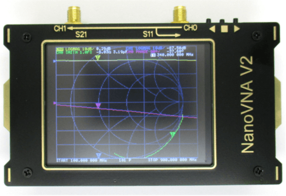
Now the antenna can be attached. In this case, it consisted of a ground plane with two radials angled downwards. Everything was made from 0.6-mm-thick silver-plated copper wire. Both the quarter-wave radiator and the two radials were exactly 10 cm long. Therefore, you can expect a wavelength of 40 cm and a frequency of 750 MHz.

 

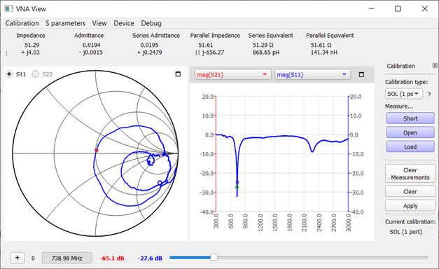
The measurement indeed shows a sharp resonance at 739 MHz. The feed point impedance is conveniently close to 50 Ω. A few small experiments demonstrated that this impedance can be adjusted by changing the angle of the two radials. Achieving an exact 50 Ω match is easily doable.

The measurement also shows a second resonance at approximately three times the frequency, the three-quarter wavelength resonance, at 2272 MHz. Here, the impedance is around 97 Ω.

One could shorten the antenna to reach a higher frequency. This is a common procedure in amateur radio: initially making the antenna slightly too long and then gradually trimming it until the resonance is at the desired frequency. Antenna measurements are one of the most frequent applications of the NanoVNA, but it can do much more.

Measuring Components

Since I’m particularly interested in shortwave, I set the frequency range to 1 MHz to 30 MHz for the following measurements. I also set 500 measurement points. This is a lot and provides good resolution, but also results in relatively slow measurements. The output power of the generator was set to −20 dBm.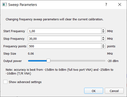

 

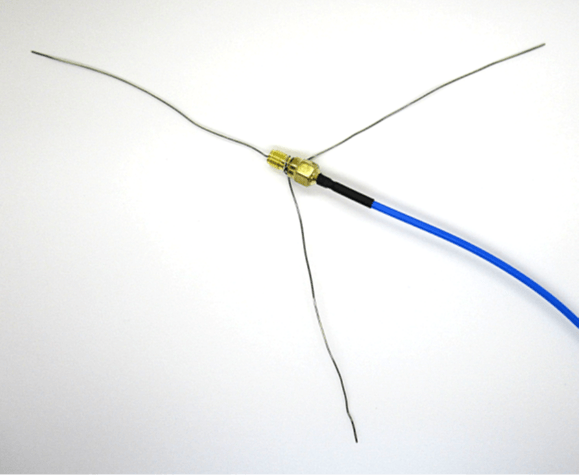
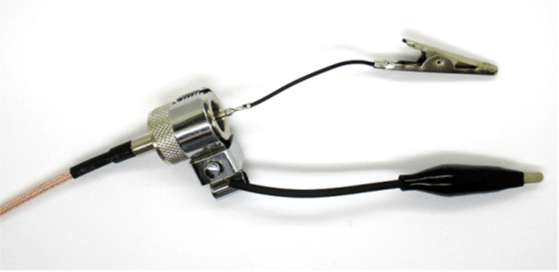
For my experiments, I made a coaxial cable with two alligator clips at the ends, with the free ends being only about 5 cm long. Up to 30 MHz, this setup works well because the connections are much shorter than the quarter wavelength of 2.5 m at 30 MHz. The additional inductances of the connections do affect the measurement, so the calibration must be done with this cable. For the standard SMA cables, there are three end caps for short circuit, open circuit, and 50 Ω load. However, with a custom cable, I can’t use them.

 

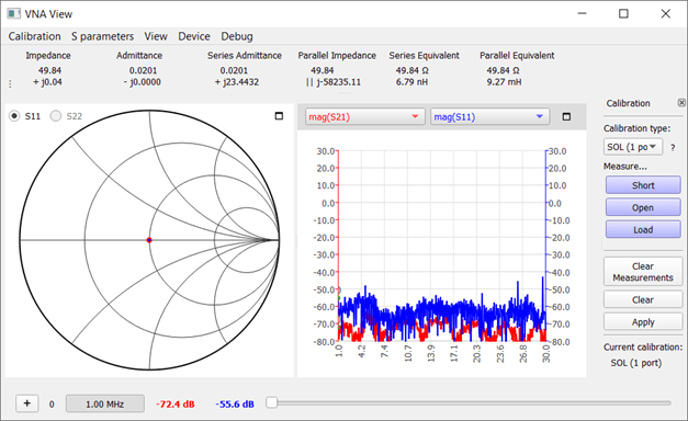
If a calibration has already been performed, the three fields ‘Short,’ ‘Open,’ and ‘Load’ appear blue. First, click on ‘Clear Measurements’ to delete the old calibration. The three fields will turn white. Then, create a short circuit at the end of the test cable, in this case by connecting the two alligator clips. Click on ‘Short.’ The device will go through all the measurement points and store the results for the short circuit condition. When finished, the ‘Short’ button will turn blue again. Then open the connection, click ‘Open,’ and wait until this field also turns blue. Finally, attach a 50 Ω resistor (51 Ω or two 100 Ω resistors in parallel will also work), click ‘Load,’ and wait until this field turns blue. After that, click ‘Apply’ to make this calibration effective for the following measurements.

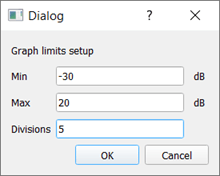
I used only the CH0 port, as in the UHF antenna measurement, to perform S11 measurements, i.e. measuring the complex impedance of components or antennas. However, the signal at CH2 is always displayed in red. Usually, you see the background noise at −70 dB here. By narrowing the measurement range, the blue CH0 channel becomes more visible, and the red channel no longer interferes. Under ‘View/Graph Limits,’ I selected −30 dB to +20 dB with five divisions.

 

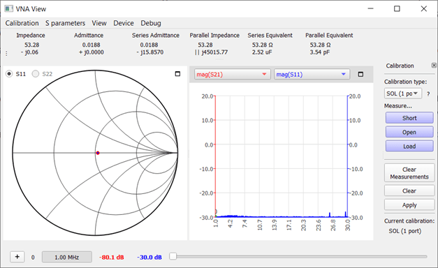
Now the actual measurements begin. Using the same resistor I used for calibration, I see a point exactly in the center of the Smith chart. The right-hand diagram, mag(S11), shows the reflected power at around −30 dB, indicating almost perfect matching. After prolonged operation, the calibration may slightly shift. Therefore, at 1 MHz, I can now read a resistance value of 53 Ω. The measured parallel capacitance of 3.5 pF is negligible.

 

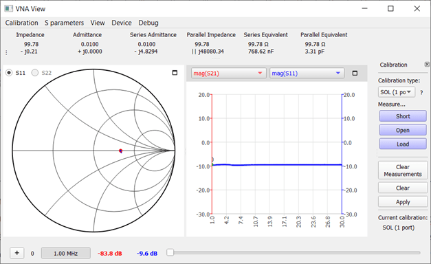
A 100 Ω carbon film resistor with was measured at 99.79 Ω. The Smith chart shows a point on the middle line, indicating that any capacitance or inductance is negligible. The return loss is consistent across the entire frequency range.

 

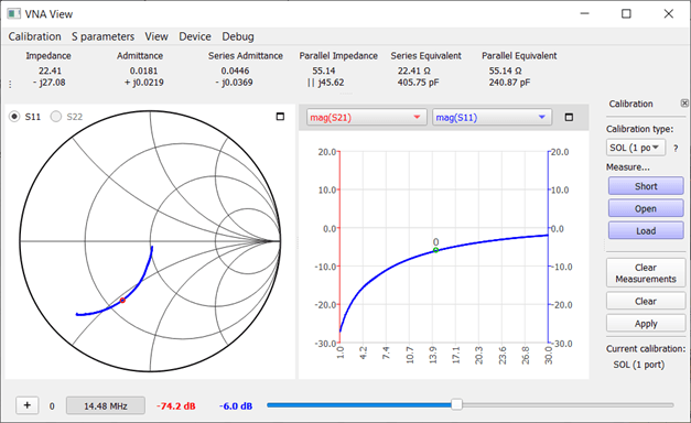
To get better acquainted with the measurements, it’s helpful to start with some well-defined objects. Therefore, a 51 Ω resistor was connected in parallel with a 220 pF capacitor. The Smith chart shows a curved line. The fact that it lies below the middle line indicates a capacitive component. The right-hand diagram shows that more power is reflected as the frequency increases. Mathematically, the capacitive reactance of the capacitor at 14.5 MHz is exactly 50 Ω. At this cutoff frequency, the return loss is 6 dB. Using the slider at the bottom, this frequency was set. It shows that the real and imaginary components of the impedance are of similar magnitude and that the capacitance, at 240 pF, is slightly larger than specified.

 

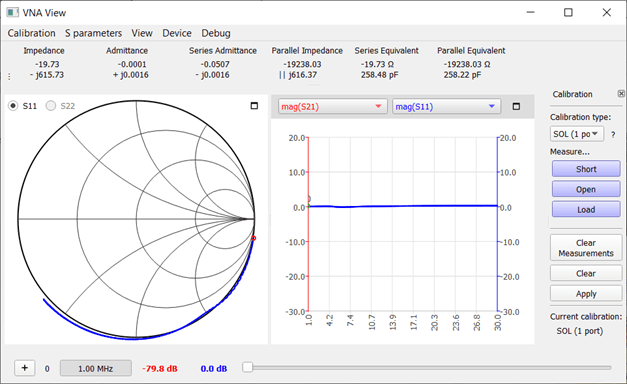
To examine a variable capacitor, it was turned to maximum capacitance, which was measured at 258 pF. The Smith chart shows a circular segment right on the unit circle. Slight deviations outward indicate that a new calibration is due. The return loss is 0 dB, meaning no losses were measured in the variable capacitor.
 

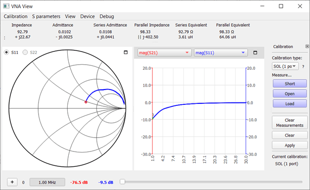
A 91-Ω, 10 W ceramic power resistor shows a strong inductive component because it contains a coiled wire resistor inside. This ‘coil’ obviously has an inductance, measured as 3.6 µH. The curve in the Smith chart is entirely in the upper half. This makes it clear that this resistor is not suitable for high frequencies.

 

In contrast, a smaller 68 Ω, 5 W power resistor showed no inductance. It can be used as a dummy load for small HF power amplifiers up to 30 MHz. However, I already have a homemade dummy load made from 24 parallel-connected 1.2 kΩ, 1 W carbon film resistors with. I also measured this, and it passed the test: a smooth 50 Ω with no reactance up to 30 MHz.

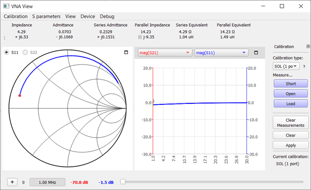
A small inductor with a nominal value of 1.1 µH was measured at 1.04 µH at 1 MHz. The series loss resistance is about 4 Ω at 1 MHz but rises to 16 Ω at 30 MHz. The losses are evident from the fact that the measurement curve in the Smith chart is clearly within the unit circle.

 

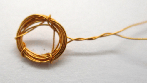
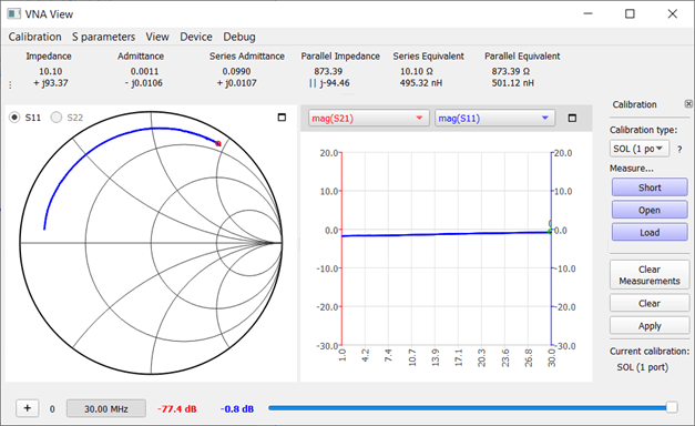
I often use simple air-core coils in low-pass filters. Ten turns of 0.2 mm enameled copper wire with a coil diameter of 5 mm should result in approximately 0.5 µH. The last turn is also used to tie the bundle together. It’s clear that this design results in greater losses. But now I can finally measure how significant these losses are.

 

At 495 nH it comes very close. However, at 30 MHz, I already see a series loss resistance of 10 Ω. At 7 MHz, it’s only 5 Ω. Roughly estimating, such a filter brings losses of about 10%. This is something I wouldn’t have discovered with my previous measurement methods. The VNA proves its worth!

 

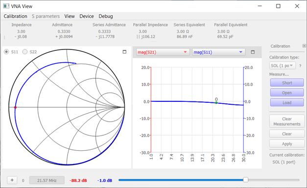
The NanoVNA can also examine cables. A coiled 50 Ω cable was connected on one end and left open on the other. The measurement shows capacitance at the lower end and inductance at the upper end. At 21.57 MHz, the curve in the Smith chart crosses the neutral centerline. This indicates the quarter-wave resonance. The electrical length of the cable is therefore 3.48 m. However, the mechanical length was only 2.95 m. From the ratio, a velocity factor of 0.86 can be calculated, meaning that waves travel through the cable at 86% of the speed of light.