The Analog Thing - The Arduino of Analog Computing?

An Analog Computer?

Unlike a digital computer that manipulates discrete binary values, an analog computer processes data represented by continuous physical quantities, such as electrical voltages or mechanical movements. Analog computers can solve complex differential equations and simulate physical systems in real-time. They were used in early aerospace and military applications, where they helped to understand complex dynamic systems and control theory.

The complexity, limited precision and limited flexibility of analog computers make them hard to use. Therefore, they have been superseded by digital computers in most applications. And this is where the Berlin-based company Anabrid comes in. Their (self-imposed) mission is to reintroduce the analog computer as a complement to the digital computer to help keep Moore’s law alive, to save energy, and to improve security. One of their tools to achieve their mission is The Analog Thing (abbreviated to THAT).

The Analog Thing Has an Intriguing User Interface (IUI)

The Analog Thing is a flat, rectangular (20 cm by 24 cm) sandwich of two white printed circuit boards (PCBs) with a height of approximately 38 mm. The lower board carries all the electronic components. The (thick) upper board provides the user interface with intriguing symbols printed in black on it. About half of its surface is reserved for a 17 × 10 patch matrix/bay/panel. Each patch hole is at the center of a graphical symbol: a circle, a diamond, or a triangle. Triangles are white, circles are white or black while diamonds come in white, black and half-white/half-black (see Figure 1).

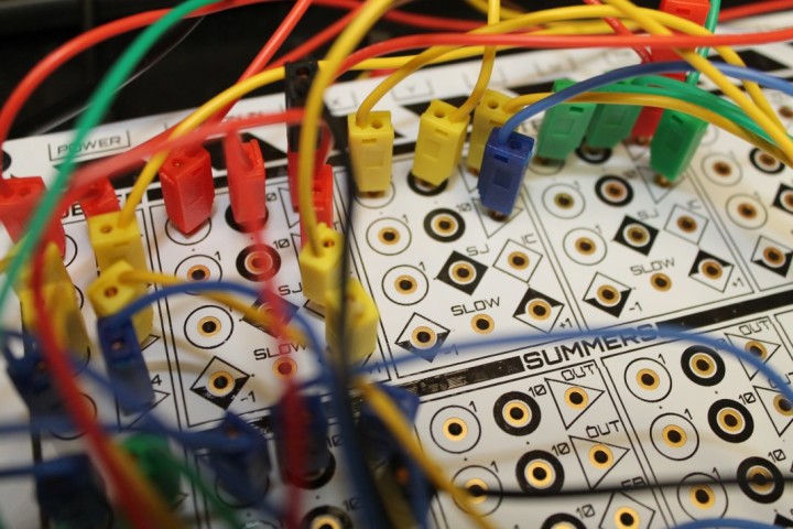
The patch panel is subdivided into 17 computing elements where each element represents a mathematical function like integrator (5×), multiplier (2×), summer (4×), inverter (4×) and comparator (2×). There are also eight coefficients and four ±1 constants.

Below the patch panel are two more rows of holes with capacitors (5×), diodes (4×), Zener diodes (2×) and four signal outputs.

The patch panel is separated from the control panel by the name of the device, printed from left to right in large characters. The control panel consists of nine potentiometers (COEFF 1 to 8 and OP-TIME) and two rotary switches (COEFFECIENT and MODE). There is also a numerical LCD panel meter, and three LEDs provide some status information.

At the top side of THAT we find all the connectors: power (USB-C, only a cable is included, not a power supply), outputs (RCA, a stereo cable is included) and extension (pin headers, one 2 × 5 flat cable is included).

Patch Cables

Like digital computers, THAT doesn’t do anything without a program. However, loading software is not a matter of connecting a thumb drive or a microSD card. Programming is done by sticking 2-mm banana-plug patch cables into the holes of the patch panel. The Analog Thing comes with 30 patch cables in five colors.

Display Not Included With The Analog Thing

The Analog Thing produces analog signals in the shape of voltages in the range of −1 V to +1 V (the precision of THAT is about 1%). A signal can be made available on four output connectors X, Y, Z and U. To visualize them, an oscilloscope or a computer with soundcard (or other analog input) is required. In many cases, you want a XY(Z) display, so the oscilloscope should have an XY(Z) mode. For optimal results, these inputs should feature DC-coupling. Therefore, a soundcard is not the best option.

THAT can output up to four signals, and so a 4-channel oscilloscope is ideal. It is therefore a bit unfortunate that the output connectors are RCA and not BNC. This was probably done to keep the costs low and make it all fit. RCA-to-BNC adapters are not included.

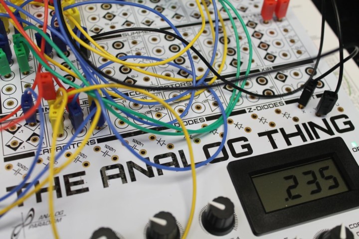
The panel meter is a 3.5-digit (±1,999 count) voltmeter (Figure 2). However, as far as I could determine, it cannot be connected to signals produced by the unit’s computing elements. Its use is to display coefficient values and show the execution speed.

Master-Minion Chaining

One last thing to mention before going into the programming of THAT is the extension option. When more computing elements are needed than are available on THAT, it is possible to connect one or more units in series. The first one will be the master, while the others are the “minions”. The number of elements in a chain is said to be unlimited.

As a side note, I have come across other attempts to remove the master-slave paradigm from electronics speak, but never this one. Even though I find it quite nice, I am not sure to adopt it, as Master and Minion both start with “M”. As an example, on a SPI bus, MISO (Master In Slave Out) and MOSI (Master Out Slave In) would both become MOMI. Maybe rename Master to “Gru”?^* Then we would get GIMO & GOMI.

* Felonius Gru is the supervillain-turned-hero helped by an army of yellow minions made popular by the “Despicable Me” movie series.

What Can You Do with THAT?

Programming The Analog Thing is not done by typing strange commands into a terminal or text editor, but by plugging cables into the patch panel. It is similar to visual programming where functional blocks are connected with virtual wires.

An analog program is a mathematical expression that describes a dynamic system, i.e. a system that evolves over time according to known relationships. So, in order to make THAT do something useful, you must first come up with a suitable mathematical model. This alone makes analog computing almost inaccessible to most mortals. Believe it or not, but differential equations are just not as popular as Python or TikTok.

Example Programs For The Analog Thing

To help you get started with analog programming on THAT, its user manual features nine examples, from mathematical curiosities to real-world applications. Each example explains the model it implements, presents the mathematical equations and its corresponding signal flow diagram, the cabling diagram (the patch), and the expected output graph.

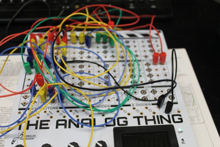
To apply a patch, you plug the patch cables on THAT according to the cabling diagram. For those who are old enough to have done it, this must be done with the same care as copying a BASIC program listing from a computer magazine in the eighties. One mistake and the program won’t work. The danger here is not so much plugging a cable in the wrong hole as the multicolor patch diagrams are quite clear, but to not forget a cable. Sifting through the patch cable spaghetti to figure out which wire is wrong or missing isn’t easy (Figure 3).

Setting Coefficients

After patching THAT, you must set the coefficients used in the patch. A coefficient is simply a “volume” potentiometer that has its input in the COEFF section. To set the value of a coefficient, set the rotary COEFFICIENT switch to the coefficient’s number (1 to 8) and set the MODE switch to COEFF. The LCD now shows the coefficient’s value. You can adjust it by turning the corresponding potentiometer. Three-decimal precision is doable (with some patience). Note how in the Lunar Landing example two coefficients are put in series to obtain even higher precision values.

Execute an Analog Program

Now it is time to execute the patch. For this, rotate the MODE switch to the OP position. The OP LED will light up. Connect a suitable display device to the outputs of THAT. The Lunar Landing example has three output signals (X, Y and U) so a 3-channel display would be best.

In OP-mode, the patch is executed once. In REP-mode, the patch is executed repeatedly. REPF-mode repeats 100× faster than REP mode. Note that every repetition is preceded by a restart of the patch as the integrators must be reset to their initial condition. This makes it complicated to create a smoothly repeating patch. Those interested in using THAT in e.g., musical applications would probably be better of with continuously evolving patches than with repeating pacthes.

Hello, Analog World!

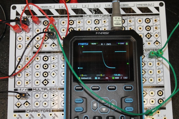
The first example from the user manual, Radioactive Decay, can probably be considered as the equivalent of the “Hello World!” example in digital computer programming. It implements a first-order differential equation well known to electronics enthusiasts as it also applies to discharging a capacitor C through a resistor R:

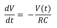
The example uses λ in place of 1/(RC) and V is called N but that doesn’t change anything.

The patch requires six wires and runs in REP mode. The oscilloscope shows a nice exponential curve representing radioactive decay (or a capacitor discharging through a resistor, see Figure 4). Potentiometer 1 controls the amplitude, potentiometer 2 controls the slope.

As a second example, I tried the Lorenz Attractor, related to the well-known Butterfly Effect (a tiny change in an early system state can result in huge differences in later states). This complex patch consumes 22 wires (see Figure 3), and six coefficients must be carefully adjusted one by one. A 2-channel (analog) oscilloscope in XY mode gives the best results. I managed to patch the program without making mistakes and was then hypnotized by the continuously changing graph.

Mainly an Educational Tool

The quality of the Analog Thing is outstanding. It is nicely made and well thought out. Patch holes, albeit simple gold-plated holes, provide good contact, even with sometimes wiggly banana-plug patch cords. The LCD panel meter’s readings are stable, and the potentiometers turn smoothly.

Electronics engineers may be attracted to THAT as they are used to circuits with integrators and other computing elements found on it. Turning a simple model into a patch diagram should be doable for certain enthusiasts but how to convert the equations of the Euler Spiral of example 9.5 needs a bit more explaining than provided in the “First Steps” booklet. Sticking in wires randomly will most probably result in frustratingly flat outputs clipping at the min or max value.

Maybe one day The Analog Thing will become the Arduino of analog computing, supported by thousands of community-made models and patch diagrams. The initial conditions for huge popularity have been set. Like Arduino, THAT is open source, and the design files can be found at GitHub. However, until takeoff, THAT is mainly an educational tool and a curiosity for people interested in playing with mathematical models. In any case, whatever you do with it, it is a great conversation starter.